
kar7mp5
[Python] Implementation of Differences (SSD) through Depth Map Sum of Squared 본문
AI/Vision
[Python] Implementation of Differences (SSD) through Depth Map Sum of Squared
kar7mp5 2024. 12. 9. 22:58728x90
௹ 양안 시차 (Binocular Disparity)
이미지 출처: OpenCV official docs
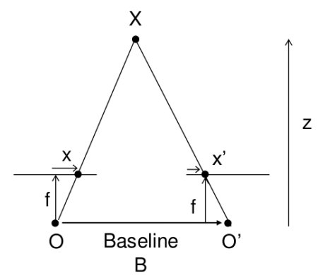
양안 시차는 인간과 같은 양안 시각 시스템에서 두 눈이 약간 다른 각도에서 대상을 보는 데서 발생하는 시각적 차이를 의미한다.
가까운 사물일 수록 시차(Disparity)가 크고, 멀리에 있는 사물일 수록 시차가 작다.
$$
disparity = x - x^\prime = \frac{Bf}{Z}
$$
$x$와 $x^\prime$: 3D 공간 상의 한 점(Scene Point)이 두 카메라에서 투영된 이미지 평면 상의 좌표
$B$: 두 카메라 센터 간의 거리 (Baseline)
$f$: 카메라의 초점 거리(Focal Length)
깊이(Depth): 3D 공간 상의 한 점(Scene Point)에서 카메라까지의 거리
௹ The Sum of Squared Differences (제곱 차 합)
기본 개념으로 왼쪽, 오른쪽 이미지가 유사하지 않을 수록 거리가 가깝고, 유사할 수록 거리가 멀다고 설명했다.
여기서 핵심은 "두 이미지 간 유사도" 라고 볼 수 있다.
필자는 이번에 MSE(평균제곱오차) 방식으로 유사도를 구하였다.
$$
SSD(x, y, d) = \sum_{i=-\frac{B}{2}}^{\frac{B}{2}} \sum_{j=-\frac{B}{2}}^{\frac{B}{2}} \left( I_L(x + i, y + j) - I_R(x + i - d, y + j) \right)^2
$$
$I_L$: 왼쪽 이미지
$I_R$: 오른쪽 이미지
$B$: Block size(블록 사이즈); 비교할 이미지 크기
$d$: Disparity(깊이)
OpenCV로 구현
from matplotlib import pyplot as plt
import numpy as np
import cv2

# Load images
imgL = cv2.imread('./data/tsukuba_l.png',0)
imgR = cv2.imread('./data/tsukuba_r.png',0)

# Compute disparity
stereo = cv2.StereoBM_create(numDisparities=16, blockSize=15)
disparity = stereo.compute(imgL,imgR)

# Display the plots
plt.imshow(disparity,'inferno')
plt.show()
Numpy로 구현
import numpy as np
import matplotlib.pyplot as plt

def compute_disparity(imgL, imgR, num_disparities, block_size):
    """
    Computes the disparity map between a pair of rectified stereo images.

    Args:
        imgL (np.ndarray): Left grayscale image.
        imgR (np.ndarray): Right grayscale image.
        num_disparities (int): Maximum disparity range to search.
        block_size (int): Size of the square block for block matching.

    Returns:
        np.ndarray: Disparity map with the same dimensions as the input images.
    """
    # Ensure the images are numpy arrays and have float32 type
    imgL = np.asarray(imgL, dtype=np.float32)
    imgR = np.asarray(imgR, dtype=np.float32)

    # Get the dimensions of the images
    height, width = imgL.shape

    # Initialize the disparity map with zeros
    disparity_map = np.zeros((height, width), dtype=np.float32)

    # Calculate half of the block size for easier indexing
    half_block = block_size // 2

    # Loop over each pixel in the left image
    for y in range(half_block, height - half_block):
        for x in range(half_block, width - half_block):
            # Define the block region in the left image
            blockL = imgL[y - half_block:y + half_block + 1, x - half_block:x + half_block + 1]

            # Initialize variables for the best match
            min_ssd = float('inf')
            best_disparity = 0

            # Search for the best disparity in the range [0, num_disparities)
            for d in range(num_disparities):
                if x - d - half_block < 0:
                    continue
                # Define the block region in the right image
                blockR = imgR[y - half_block:y + half_block + 1, x - d - half_block:x - d + half_block + 1]

                # Compute the sum of squared differences (SSD) between blocks
                ssd = np.sum((blockL - blockR) ** 2)

                # Update the best disparity if SSD is smaller
                if ssd < min_ssd:
                    min_ssd = ssd
                    best_disparity = d

            # Assign the best disparity value to the disparity map
            disparity_map[y, x] = best_disparity

    return disparity_map

# Load grayscale images as numpy arrays
imgL = plt.imread('./data/tsukuba_l.png')
imgR = plt.imread('./data/tsukuba_r.png')

# Ensure the images are 2D arrays (grayscale)
if imgL.ndim == 3:
    imgL = imgL[:, :, 0]  # Convert to grayscale if needed
if imgR.ndim == 3:
    imgR = imgR[:, :, 0]  # Convert to grayscale if needed

# Parameters for disparity computation
num_disparities = 16
block_size = 20

# Compute the disparity map
disparity = compute_disparity(imgL, imgR, num_disparities, block_size)

# Visualization of the results
plt.figure(figsize=(10, 3))

# Original image
plt.subplot(1, 2, 1)
plt.imshow(imgL, cmap='gray')
plt.title('Original Image')
plt.axis("off")

# Disparity map
plt.subplot(1, 2, 2)
plt.imshow(disparity, cmap='inferno')
plt.colorbar()
plt.title('Disparity Map')
plt.axis("off")

# Display the plots
plt.show()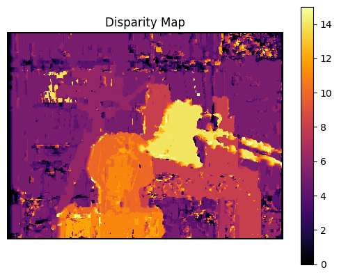
728x90